Introduction

In our nervous system, we have neurons, connected by axons and dendrites. The connecting regions are called synapses. And when a stimuli occurs, these neurons fire and the strength of the synaptic regions changes. This is our process of learning - artificial neural networks imitate this process.

General Overview
Single-layer Neural Network
Loss function
Gradient Descent
Activation Functions

General Overview

The computational units neurons are connected to one another through weights. Each input to a neuron is scaled with a weight, which affects the function computed at that unit. A neural network is a collection of neurons connected by weights, propagating the input through the network to compute the output. Learning occurs by changing the weights between neurons.

Consider a dataset $\mathbb{D} = \{(x^{(i)}, y^{(i)}) | 1 \leq i \leq m, x \in \mathbb{R}^d, y \in \mathbb{R}\}$ . Each training instance is fed into the neural network so that it can make predictions about the output label. Depending on how well the neural network did, the weights are adjusted. By changing the weights, we hope to make better predictions in the future. Eventually, over many iterations, we would like to reach a point where the neural network, trained on the training data, is able to make accurate predictions on unseen test data. This is called generalization.

Single-layer Neural Network

This is the simplest neural network. It has $1$ input layer (not counted) and $1$ output node. Consider a training instance of the form $(x^{(i)}, y^{(i)})$ , where each $x^{(i)} = [x_1^{(i)},...,x_d^{(i)}]$ contains $d$ features, and $y^{(i)} \in \{ -1, +1 \}$ is an observed binary value. The input layer contains $d$ nodes representing the $d$ features with edges of weight $W^T = [w_1,...,w_d]$ connecting the input nodes to the output node. In addition, there is often a bias term $b$ (the invariant part of the prediction) included. The bias term is a constant value that is added to the linear function. The bias term is represented by a node, called the bias neuron with a constant value of 1, and an edge of weight $b$ connecting it to the output node.

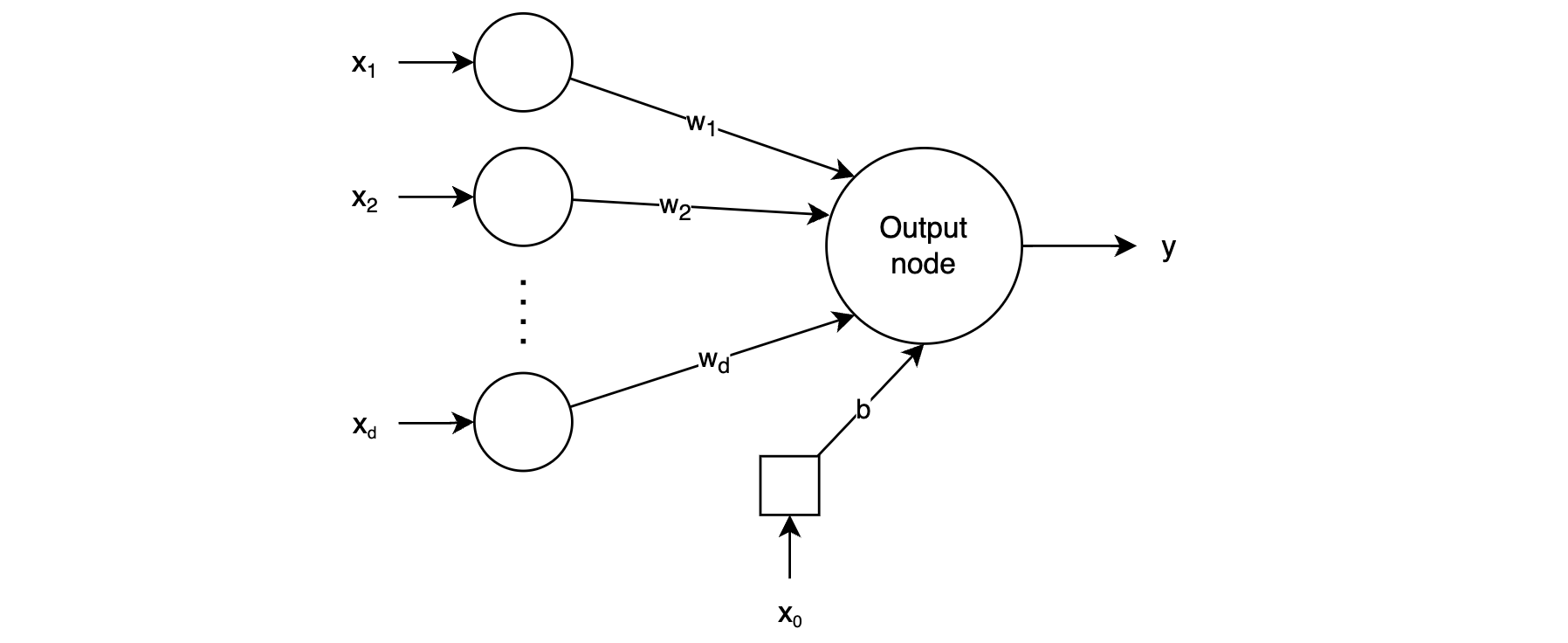
At the output node, the linear function is $x^{(i)}W + b = \sum_{j=1}^d w_j x_j + b$ . The output of the network is the sign of the linear function (here $i$ corresponds to the training instance index and $j$ corresponds to the feature index):

\hat{y}^{(i)} = \text{sign}(x^{(i)}W + b) = \text{sign}(\sum_{j=1}^d w_j x_j^{(i)} + b)

The error can then be calculated as:

\epsilon^{(i)} = y^{(i)} - \hat{y}^{(i)}

Loss function

The loss function measures how well the model is performing based on the training data. In general, we would like to minimize misclassifications or loss. For binary classification with outputs in the set $\{-1, +1\}$ , the cross-entropy loss is:

L = - \sum_{(x^{(i)}, y^{(i)}) \in \mathbb{D}} y^{(i)} \log(\hat{y}^{(i)}) + (1 - y^{(i)}) \log(1 - \hat{y}^{(i)})

Where $\hat{y}^{(i)}$ is the predicted probability of the positive class (i.e., $y = +1$ ).

Our goal would then be to minimize this loss function:

\text{argmin}_W L

To minimize this function, we can use the first derivative or its gradient to find/approach the minimum.

Gradient Descent

Gradient descent is an iterative optimization algorithm used to find the values of the weights $W$ that minimize the loss function $L$ . The general idea is to compute the gradient of the loss function with respect to each weight, and then adjust the weights in the direction of the negative gradient. This process is repeated until the loss converges to a minimum value or until a specified number of iterations is reached.

For the cross-entropy loss, the gradient with respect to the weights $W$ and bias $b$ can be derived based on the specific activation function used. The general update rules in gradient descent are:

W = W - \alpha \frac{\partial L}{\partial W}

b = b - \alpha \frac{\partial L}{\partial b}

Where $\alpha$ is the learning rate, a hyperparameter that determines the step size of each iteration. By iterating this update rule, the algorithm adjusts the weights and biases to minimize the cross-entropy loss and improves the model's performance on the training data.

Types of Gradient Descent

Batch Gradient Descent (BGD)
- Description: In BGD, the gradient is calculated using the entire training dataset. This means that for each iteration, we use all the training examples to compute the gradient of the loss function.
- Update Rule: $W = W - \alpha \sum_{i=1}^N \frac{\partial L^{(i)}}{\partial W}$ $b = b - \alpha \sum_{i=1}^N \frac{\partial L^{(i)}}{\partial b}$
- Advantages:
  - Stable convergence.
  - Straightforward implementation.
- Disadvantages:
  - Can be very slow for large datasets as it processes all training examples for each iteration.
  - Requires the entire dataset to be in memory.
Stochastic Gradient Descent (SGD)
- Description: Instead of using the entire dataset, SGD updates the weights using only a single training example at a time.
- Update Rule: $W = W - \alpha \frac{\partial L^{(i)}}{\partial W}$ $b = b - \alpha \frac{\partial L^{(i)}}{\partial b}$
- Advantages:
  - Faster than BGD, especially for large datasets.
  - Can escape local minima due to its noisy updates.
- Disadvantages:
  - Can lead to oscillations in convergence due to the noisy updates.
  - Less stable convergence compared to BGD.
Mini-Batch Gradient Descent (MBGD)
- Description: A compromise between BGD and SGD. It updates the weights using a small random subset (mini-batch) of the training dataset. The size of the mini-batch is typically between 10 and 1000.
- Update Rule: $W = W - \alpha \sum_{i \in \beta} \frac{\partial L^{(i)}}{\partial W}$ $b = b - \alpha \sum_{i \in \beta} \frac{\partial L^{(i)}}{\partial b}$
- Advantages:
  - Can be faster than both BGD and SGD, especially for large datasets.
  - Benefits from both the stability of BGD and the faster convergence of SGD.
  - Can be implemented efficiently on parallel hardware (like GPUs).
- Disadvantages:
  - Convergence is less stable than BGD but more stable than pure SGD.

MBGD is the most used variant. The choice of batch-size $\beta$ and learning rate $\alpha$ are hyperparameters that influence speed and stability of convergence.

Activation Functions

In the case of our single-layer classifier, our activation function was the sign function. And this makes sense, given that a binary class label needs to be predicted. However, there are many different types of situations where different target variables need to be predicted.

If we want to predict a continuous value, we would need a different activation function, such as an identity activation function. The resulting neural network would just be a linear regression model. If we want to predict a probability, we would need a sigmoid activation function. If we want to predict a class label, we would need a softmax activation function. For different situations, there are different activation functions. This is crucial when considering multi-layered neural networks. If a network only used linear activations, then it would be the same as using a simple linear regression model.

The greek letter $\bm{\phi}$ denotes an activation function:

\hat{y} = \bm{\phi}(x^{(i)}W + b)

Technically, a neuron calculates two functions. First, the linear function $x^{(i)}W + b$ value is calculated. Then, the activation function $\bm{\phi}$ is applied to the result of the linear function. The resulting values are called the pre-activation and post-activation values, respectively.

Activation Function	Equation	Range
Identity	$\bm{\phi(z) = z}$	$(-\infty, \infty)$
Sigmoid	$\bm{\phi(z) = \frac{1}{1 + e^{-z}}}$	$(0, 1)$
Tanh	$\bm{\phi(z) = \frac{e^z - e^{-z}}{e^z + e^{-z}}}$	$(-1, 1)$
Rectified Linear Unit (ReLU)	$\bm{\phi}(z) = \max(0, z)$	$[0, \infty)$
Hard Tanh	$\bm{\phi}(z) = \max(-1, \min(1, z))$	$[-1, 1]$
Softmax	$\bm{\phi(z) = \frac{e^{z_j}}{\sum_{k=1}^K e^{z_k}}}$	$(0, 1)$

ReLU is used most widely used for the advantages it offers:

More computationally efficient (no exponentials)
Has a gradient of either $0$ (for negative values) or $1$ (for positive values), which helps mitigate the vanishing gradient problem
Inherently introduces sparsity (many neurons will have a value of $0$ ), which can reduce overfitting

ReLU does have the "dying ReLU" problem. This refers to the problem where neurons in a network can sometimes output a constant zero value for all inputs — essentially becoming inactive and no longer updating during training. This can be mitigated by using leaky ReLU, where $\alpha$ is a small constant ( $0.1$ , $0.01$ , etc.):

\bm{\phi}(z) = \text{max}(\alpha z, z)

Softmax

There is a bit more to say about softmax. If we would like to classify an input among $k$ classes, it becomes a multi-class classification problem. In this case, $k$ output values $o = [o_1,...,o_k]$ can be used, such that the activation function for the $i$ th output node is:

\bm{\phi}(o_i) = \frac{e^{o_i}}{\sum_{j=1}^k e^{o_j}}

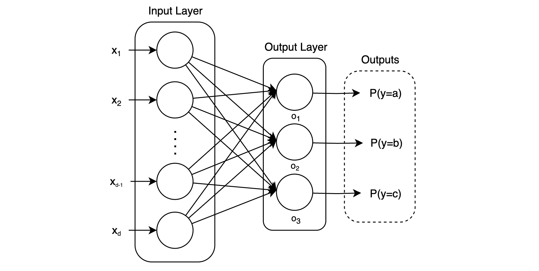
The softmax function is used to normalize the output values to be between $0$ and $1$ , representing the probability of each class given the input.

L(y, p) = -\left( y \log(p) + (1-y) \log(1-p) \right)

L = \log(1 + \exp(-y \hat{y}))