Introduction

• Datasets
• Architecture
• Experimental Design
• Results
• Discussion
• References

In long-term time series forecasting (LTSF), a debate has emerged regarding the effectiveness of transformer-based models, specifically the Autoformer, versus simpler linear approaches like the DLinear model. Traditional transformer models are praised for their semantic correlation extraction capabilities in various domains but face scrutiny in their ability to capture temporal relationships essential in time series data. This contention is fueled by contrasting claims: the Autoformer's reported superiority in handling complex temporal patterns through its novel Decomposition and Auto-Correlation mechanisms ("Yes, Transformers are Effective for Time Series Forecasting (+ Autoformer)" REF), and recent empirical evidence suggesting the unexpected effectiveness of the simpler LTSF-Linear models in various real-life datasets ("Are Transformers Effective for Time Series Forecasting?" REF). Our research delves into this mystery, attempting to the uncover the truth of whether the advanced, yet computationally intensive, transformer models are really necessary for time series forecasting or if simpler models could suffice, offering comparable, if not superior, performance.

Datasets

Our investigation covers a number of mainstream time series forecasting applications: electricity consumption, traffic flow, weather patterns, exchange rate and stock market data in financial markets, to provide a comprehensive evaluation. These datasets, multivariate in nature, are a testing ground to compare the predictive abilities of Autoformer and DLinear models across different contexts. Electricity (REF) dataset contains the hourly electricity consumption of 321 customers from 2012 to 2014. Traffic (REF) is a collection of hourly data from California Department of Transportation, which describes the road occupancy rates measured by different sensors on San Francisco Bay area freeways. Weather (REF) is recorded every 10 minutes for 2020 whole year, which contains 21 meteorological indicators, such as air temperature, humidity, etc. Exchange (REF) records the daily exchange rates of eight different countries ranging from 1990 to 2016. Stock market (REF) is a collection of daily stock prices of a number of companies from 2005 to 2017.

Architecture

The cornerstone of our research is the comparative study of two distinct model architectures: the Autoformer and DLinear. Each model has a different approach to handling time series data. The autoformer has a series decomposition block, which dynamically separates time series into trend-cyclical and seasonal components. This block adapts to both historical data and predicted future trends, offering a more nuanced analysis over time. Complementing its decomposition, Autoformer also utilizes an Auto-Correlation mechanism, diverging from traditional self-attention. It focuses on period-based dependencies, clustering similar sub-series through calculated series autocorrelations, a method grounded in stochastic process theory.

Dlinear is a combination of decomposition and linear layers. It first decomposes raw data into a trend component using a moving average kernel and a residual (seasonal) component. Post-decomposition, DLinear applies one-layer linear transformations to each component (trend and seasonal) independently. The final forecast is obtained by summing the outputs of these linear layers. This method, while simpler, effectively enhances performance, particularly in datasets with prominent trends.

The Autoformer's architecture, with its inherent sparsity and sub-series-level aggregation, boasts computational efficiency and advanced temporal relationship analysis. DLinear, with its less complex structure, offers an efficient alternative, especially in scenarios where data exhibits clear trends. The Autoformer and DLinear embody contrasting philosophies in time series forecasting - the Autoformer's sophisticated architecture is designed for intricate pattern recognition and efficiency, while DLinear leverages simplicity and explicit trend handling for effective forecasting.

Experimental Design

Our experimental goal was twofold: to replicate the results claimed in the Hugging Face post advocating for Autoformer and the general effectiveness of transformer models for TSF, and to juxtapose these findings with those from the Linear LTSF paper, which argues the superiority of DLinear.

For experiment parameters, we tested with the simplest transformer model configurations, starting with 2 encoding and 2 decoding layers, followed by a variant t 2 encoding and 1 decoding layer. This approach aimed to assess the fundamental impact of encoding and decoding layers on forecasting accuracy. Then, we conducted tests on the wide-range of time-series datasets. This variety allowed for a comprehensive evaluation of model performance across different forecasting scenarios. We also included oth fixed positional embeddings and learned temporal embeddings to explore their influence on each model's capacity for temporal data processing and pattern recognition. We used the Adam optimizer with batch-size set to 16 and learning rate to ranging from 0.005 to 0.0005. We standardized sequence lengths at 336 and prediction lengths at 24, providing a uniform basis for evaluating each model's adaptability and forecasting efficacy in varied horizons.

A critical challenge we faced was the divergence in tools used in the studies we aimed to replicate. The Hugging Face post relied on the GluonTS library, a Python package for probabilistic time series modeling, developed on PyTorch and MXNet. In contrast, the Linear LTSF paper utilized PyTorch and proprietary evaluation methods.

Results

For the core performance metrics, we focused on Mean Squared Error (MSE) and Mean Absolute Scaled Error (MASE) as our primary metrics to evaluate the forecasting accuracy of the models. MSE is a standard measure of the average squared difference between the predicted and actual values, while MASE is a scale-independent metric that compares the forecasted values to a naive baseline model. Unexpected Superiority of Simplicity: Contrary to the claims favoring Autoformer in the Hugging Face blog, our replicated experiments consistently showcased the DLinear model's superior or comparable performance. This trend was observed across a majority of datasets and experimental settings.

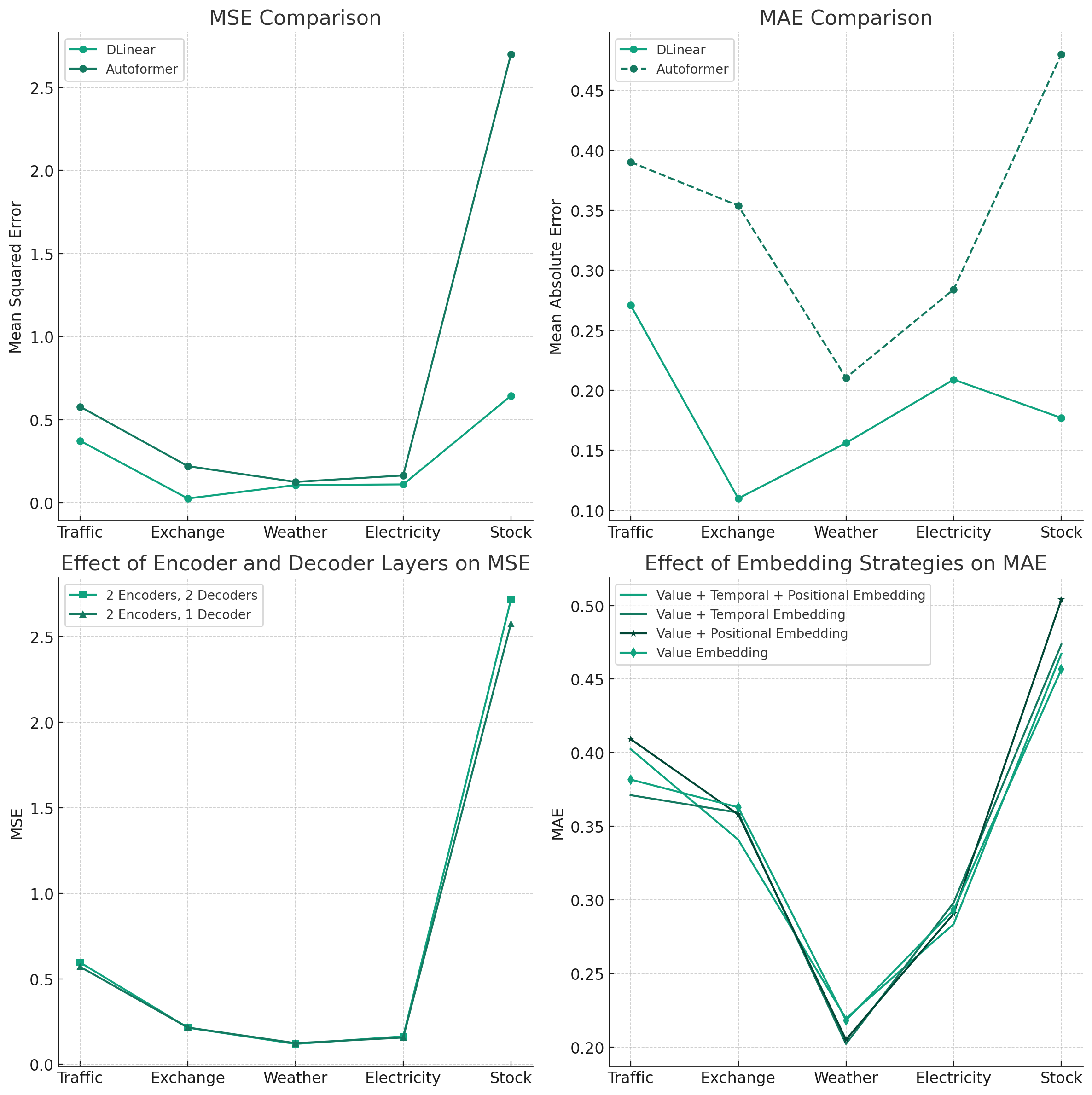
Aligning with LTSF Findings, our results echoed the sentiments of the Linear LTSF paper, underscoring the potential efficacy of simpler, linear models in time series forecasting, particularly in data scenarios marked by clear trends. As for implications for transformer ddoption, while our findings support the Linear-LTSF paper bringing a degree of skepticism to the rapid incorporation of transformer models into various fields, they also highlight that such complex models could still hold potential for future applications. However, the considerable computational resources and model complexity required to train transformers like Autoformer warrant a thoughtful consideration of their practicality and efficiency.

Discussion

Our experiments were designed to replicate, validate, and reconcile the differing claims from the two primary sources. This approach was crucial in providing a comprehensive understanding of the models' capabilities. The outcomes of our comparative analysis invite a reevaluation of the necessity for complex architectures in time series forecasting. It suggests that a simple model, such as DLinear, can be not only sufficient but potentially more effective in certain scenarios. In conclusion, our research serves as a critical examination of the current trend towards increasingly complex models in time series analysis. Wwhile advanced models like Autoformer offer sophisticated approaches, the effectiveness, efficiency, and practicality of simpler alternatives like DLinear cannot be overlooked. This realization makes the avenues for future research, balancing between model complexity and computational feasibility a lot more interesting.

References

1. Wu, H., Xu, J., Wang, J., & Long, M. (2022). Autoformer: Decomposition Transformers with Auto-Correlation for Long-Term Series Forecasting. arXiv preprint arXiv:2106.13008.
2. Zeng, A., Chen, M., Zhang, L., & Xu, Q. (2022). Are Transformers Effective for Time Series Forecasting?. arXiv preprint arXiv:2205.13504.
3. Hugging Face Blog. (2023, June 16). Autoformer. [Online]. Available: https://huggingface.co/blog/autoformer
4. Kaggle. (Updated 6 years ago). Stock Time Series Dataset (2005-2017). [Online]. Available: https://www.kaggle.com/datasets/szrlee/stock-time-series-20050101-to-20171231
5. Trindade,Artur. (2015). ElectricityLoadDiagrams20112014. UCI Machine Learning Repository. https://doi.org/10.24432/C58C86.
6. Guokun Lai. (2017). Multivariate Time Series Data. [Online]. Available: https://github.com/laiguokun/multivariate-time-series-data. [Accessed: 2023].